
Executive Summary
Hyperbolic operates an AI infrastructure platform that turns fragmented, heterogeneous bare-metal compute into a unified, productive AI cloud. We reached over $80 million of annualized run-rate revenue exiting September 2026, from essentially zero in June 2025.
A financial market for compute is arriving. Exchange-traded contracts referencing GPU rental prices are coming, and compute is following the path every commodity has taken from bilateral deals to a traded benchmark. What that layer still lacks is the physical foundation beneath it — provisioning, delivery, benchmarking and settlement against real capacity. That is what the Hyperbolic platform can provide including physical settlement.
The order of market development matters. Indices and cash-settled contracts can be built by anyone with a data feed, and several are being built now. Physical settlement cannot. It requires vetted supply, a control plane that can deliver a specific cluster on a specific date, and the counterparty relationships that make delivery enforceable. That is a platform business, not a data business, and it is the one Hyperbolic is building.
That platform is also what makes market-making in compute possible. Controlling physical settlement means controlling how capacity is packaged: the same cluster can be sold whole and long, the way it was financed, or sliced into short-duration on-demand and reserved units and sold to many buyers at once. Short duration is where the premium sits, so being able to create it at will is what turns an infrastructure position into a tradable book. Capacity locked into multi-year contracts is illiquid by construction, and standing ready to sell it in weeks or months rather than years is what makes markets and provides liquidity to the illiquid market.
Executing that conversion takes three capabilities at once. Capital alone cannot source quality capacity, and GPUs alone cannot be sold in short duration without a go-to-market engine and a virtualization layer that slices clusters and reclaims capacity between jobs. Hyperbolic runs the supplier relationships, the control plane and the demand together, which is what lets Hyperbolic capture the premium short-term pricing rather than the long-term contract rate. That premium is structural: neocloud lenders require contracted off-take, so the industry’s ability to serve short-duration demand stays limited while that demand keeps growing. We explore both arguments below.
The reference transaction is a 36-month, 256-GPU B300 supply contract carrying $28.9 million of total commitment with $5.79 million prepaid deposit. Unhedged, the base case returns 2.10× over roughly three years at a 72.3% IRR. The risk is one-dimensional: cost is fixed and contracted while the only material exposure is the price on the non-idle portion of GPU-hours. That exposure is hedged with an outright put bought against the final year of the contract. The put is not designed to pay in the base case, where it costs 0.39× and takes the base case to 1.71× at a 59.1% IRR. What it buys is the tail protection. We examine both sides of that trade below.
Physical Layer
Hyperbolic aggregates supply from neoclouds, enterprise idle capacity and customer resale into one unified control plane, and sells it as on-demand clusters, reserved capacity and private cloud with full cloud offerings including Kubernetes, Slurm, inference, orchestration, etc. Underlying the full tech stack is Forge, which virtualizes GPU clusters with different networking topology and enables buying, selling and orchestration of compute in one unified control plane. Customers land on on-demand and expand into reserved commitments as workloads become predictable and value-added services create the stickiness of the platform.
What executing this trade requires
The trade described in this paper requires three capabilities at once, and each is a business in its own right. Capital by itself does not get there: a balance sheet with no supplier relationships cannot source capacity on contract terms.
GPUs by themselves do not get there either, because owning hardware is not the same as being able to sell it. Short-duration compute needs a go-to-market engine that reaches thousands of buyers rather than a handful, and a virtualization and scheduling layer that can slice a cluster into on-demand and reserved units, place workloads across heterogeneous hardware, and reclaim capacity between jobs. Without that, a cluster can only be sold the way it was bought — whole and long.
Hyperbolic runs all three: the supplier relationships that source the capacity, the control plane that makes it sellable in short duration, and the demand that absorbs it. That combination is what lets capital deployed into this trade earn premium short term pricing rather than the long term contract rate.
The team is deliberately built at the intersection of cloud infrastructure and markets. Our CEO completed a Berkeley mathematics PhD in two years (fastest in history of Berkeley) and conducted quantitative research at Citadel Securities. Our advisors include the former Global Head of Systematic FICC at Citadel Securities and co-founders of Databricks and Lepton AI.
What power markets suggest about compute
Electricity took roughly thirty years to travel from vertically integrated utilities to tradable regional benchmarks on CME and ICE. Its structure maps onto compute closely: individual data centers are the generators, each settling at its own node defined by hardware class, vendor and location, while Hyperbolic does the work of the compute grid — aggregating heterogeneous supply into a single control plane and clearing it against demand.
The lesson that matters most here is which benchmarks won. In power, and in oil before it, the reference prices that came to define the asset class were the ones attached to the deepest physical delivery infrastructure. Indices, exchanges and lending formed around the venue where physical settlement was most liquid — not the other way around.
The end shape is clear. The winner runs robust physical settlement, produces an index as an emergent property of its own order book, and builds a hedging venue on top of that index. What is contested is the order — whether to start from physical settlement, from an index, or from a trading venue. Hyperbolic starts from physical settlement deliberately: it is the layer that cannot be bought, and the one the others attach themselves to.
Reference Transaction
The structure below is a theoretical 36-month B300 supply contract, presented as the template for a repeatable program.
Contract and capital structure
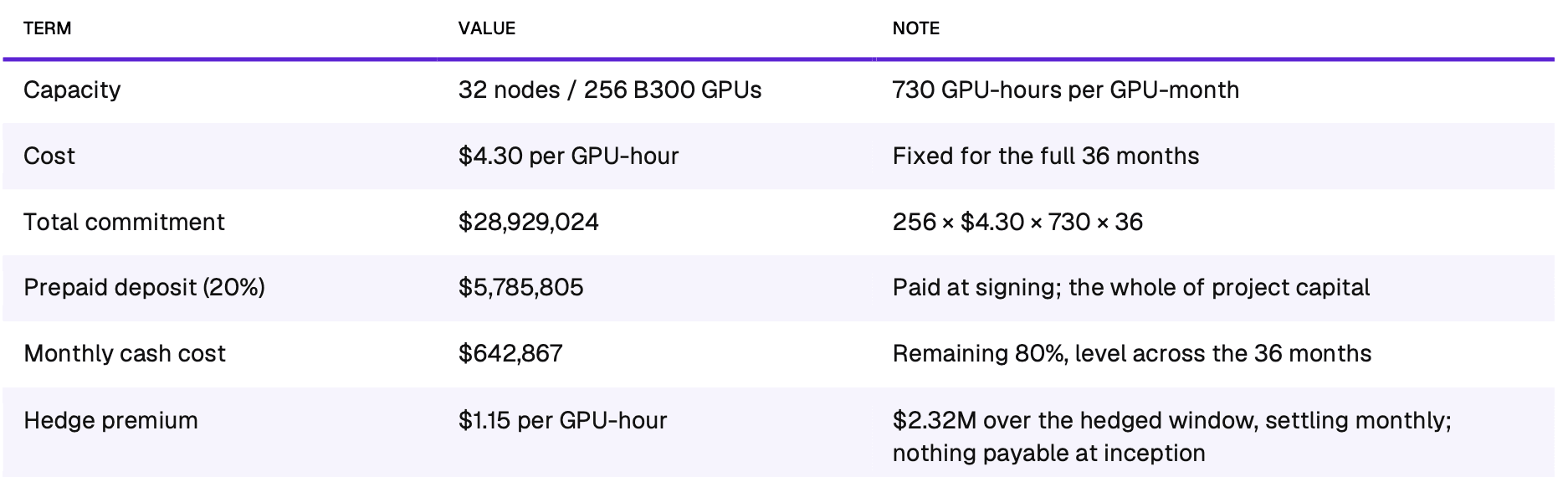
Capacity is assumed to be sold across on-demand at 65% of the fleet, short-term reserved at 25%, and 10% assumed idle. The model carries no off-take in this case, though an off-take tranche could be added to reduce the upfront capital outlay.
Why the short-duration premium persists
The pricing above assumes a durable premium for short-duration compute. That premium is a function of how the supply side is financed rather than a temporary dislocation. Neoclouds build with debt, and their lenders underwrite against contracted revenue: capacity is pledged to long-dated off-take because that is what makes the facility financeable in the first place. The result is an industry structurally biased toward selling long term, to a small number of large counterparties.
Demand does not have that shape. Training runs, evaluation cycles, inference bursts and research workloads want capacity in weeks rather than years, and want the option to stop. So the constraint on short-duration supply is not that operators have overlooked the opportunity; it is that their creditors will not let them take it. As long as lenders require contracted off-take, the industry's capacity to serve short-duration demand stays limited while that demand keeps growing, and whoever can serve it earns the spread.
Revenue and returns
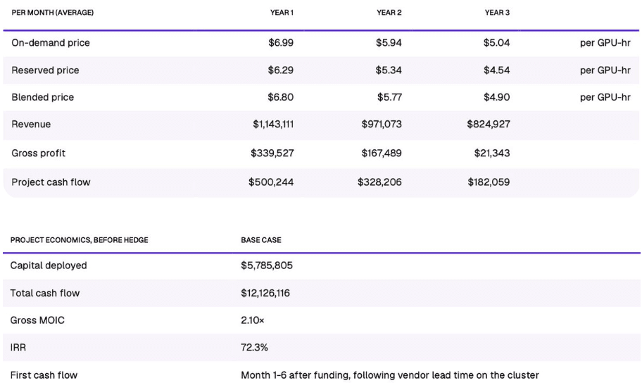
Cash flow begins as soon as the cluster is delivered and revenue starts. The model assumes four months between funding the deposit and first revenue; that gap is vendor lead time on the cluster, not a ramp on our side, and where capacity is available sooner, revenue begins sooner. Cash flow is strongest in the first year and declines with the on-demand price. The figures above carry no hedge; we examine the cost of the hedge in the hedging analysis below.
Sensitivity to Compute Pricing
Because cost is fixed for the full term, the return is driven by a single variable: the realized price on monthly GPU-hours.

The plan assumes on-demand prices decay monthly based on the decay distribution the hedging framework is scored against rather than a point forecast. The three cases below illustrate three different scenarios. The probability shown is the chance of a decay at least that severe.
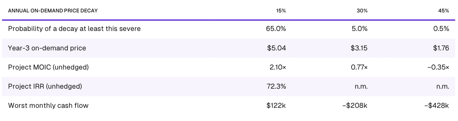
The project is robust in the first case and fails in the tail. Two-thirds of the distribution sits at a decay of 15% a year or milder, where capital is returned twice over. In the middle case, the project returns roughly three-quarters of capital; in the last case, it loses a third of it outright and runs negative cash in 22 of 36 months. Timing matters as much as depth: the probability that a given year turns cash-negative is nil in Year 1 and ~0.5% in Year 2, but ~14% in Year 3. The exposure is concentrated, late, and therefore hedgeable in a defined window.
Hedging Program
Price exposure is hedged under a defined framework rather than negotiated deal by deal. We size the structure from the project economics and a stated view of risk, and the decision rule is fixed before any dealer quote is seen. The description below is the framework.
The instrument
The structure is an outright put on the compute price. It settles monthly against an agreed upon index. The model adjusts the index by a flat basis to the blended on-demand and reserved price we actually realize to account for basis risk, and the premium settles monthly out of contract revenue with nothing payable at inception.
How the structure is chosen
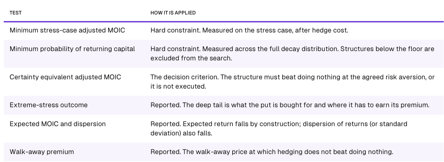
There are three decision variables: the strike, the month the hedge starts, and how many months it runs. Each candidate is scored on its certainty equivalent across a probability distribution of annual price-decay paths. The risk-aversion parameter is set before any quote is looked at, so the answer cannot be reverse-engineered from the price we happen to be offered. The bar every structure has to beat is the certainty equivalent of doing nothing.
The hedge window is determined from the cash-flow profile rather than from judgement. A year is flagged when the probability that it turns cash-negative reaches a pre-determined threshold. The strike is bounded above by the lowest base-case settlement price across the hedged months: above that line the put is already in the money in the base case, which is equivalent to pre-paying to lock a price rather than buying protection.
The framework also produces a walk-away premium — the most that can be paid before the hedged position stops beating the unhedged one. Separately, we reprice every quote against our own curve to ensure we are not overpaying.
Hedge scorecard
Two hard constraints govern the search, both measured on the stress case. Any strike that breaches either is excluded however well it scores on certainty equivalent. Adjusted MOIC throughout means total project cash flow after hedge premium and settlement, over the deposit.
Basis
Settlement references a published index while revenue is earned on our own realized prices, and the gap between the two is carried in the model as a flat basis adjustment. Because the payoff is uncapped, a wider basis does not disable the hedge: it shifts the effective strike, reducing the payout in a given month without changing the shape of the protection. Hyperbolic’s transaction data across on-demand, reserved and secondary trades relative to the index measures that gap directly.
Simulation
The project is scored against a discrete set of decay outcomes using a Monte Carlo simulation of 60,000 price paths. Each path draws its own long-run decay rate from the decay distribution, then walks month to month at 5% annual volatility, so the simulation captures the order in which prices arrive rather than only where they end up. That 5% is not a mild assumption. It sits on top of the decay distribution rather than replacing it: the structural decline in compute pricing is already carried by the decay outcomes that span a 5% annual rise to a 45% annual fall. The volatility parameter measures only the month-to-month dispersion around whichever path a scenario draws.
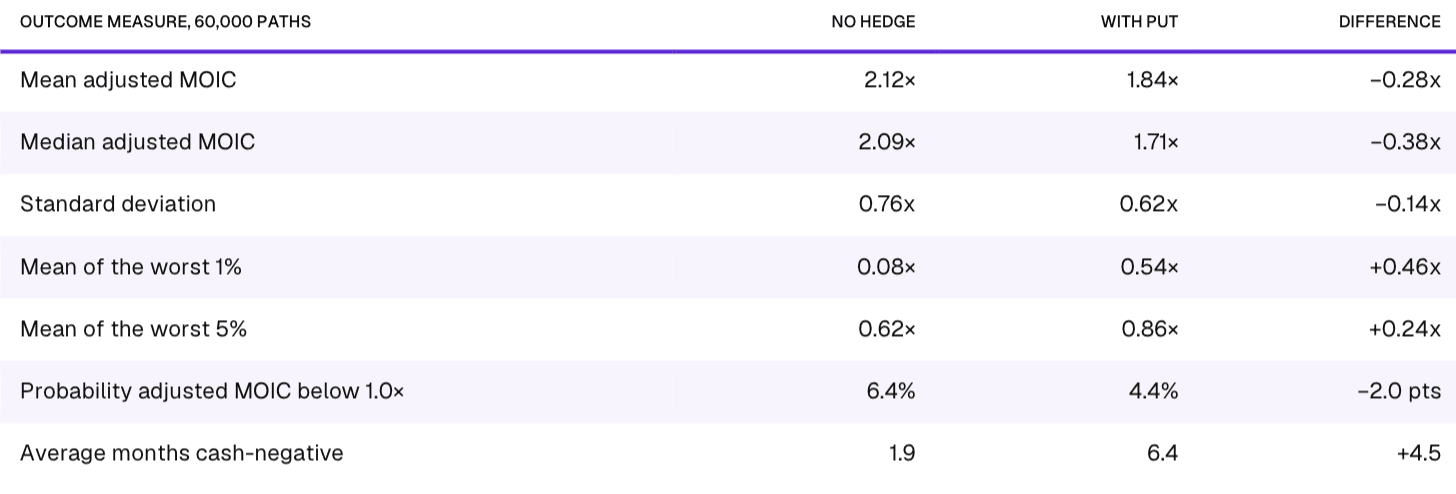
The put costs 0.28× of mean adjusted MOIC and 0.38× at the median, and returns 0.46× at the mean of the worst 1% and 0.24× at the mean of the worst 5%. The improvement grows as outcomes worsen, which is the defining property of a tail hedge: the further the price falls, the more the option pays. It also cuts dispersion, with the standard deviation falling from 0.76× to 0.62×.
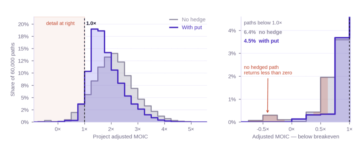
Distribution of project adjusted MOIC across 60,000 simulated price paths. Right-hand panel magnifies the region below breakeven
Conclusion
While capacity is still financed through long-dated off-take and sold the way it was financed, the gap between how supply is contracted and how demand is shaped stays wide. The trade described here is the simplest expression of that gap: buy capacity on multi-year terms at a contracted rate, sell it in short duration at premium rates, and hedge the back end where price visibility is the weakest.
What the trade requires is the ability to source capacity on contract terms, go-to-market engine to sell it in short duration, and effective hedging. Hyperbolic is well positioned to execute this trade and make markets in physical compute. We welcome questions and/or feedback from anyone to discuss further or chat about markets in general.
Disclaimer
This document is provided for discussion purposes only and does not constitute an offer to sell or a solicitation to buy any security or financial instrument, nor investment, legal, tax or accounting advice. Financial projections reflect assumptions, including the on-demand premium and idle rate; actual results will differ, potentially materially. The hedging program described is indicative only; instruments, ratios and strike levels would be determined at execution and remain subject to the existence of a liquid market.


